The Climate State of the Holocene and Anthropocene (Rates of Change)

The Anthropocene represents a new trajectory for Earth’s systems, away from a stable Holocene state.

Abstract

We explore the risk that self-reinforcing feedbacks could push the Earth System toward a planetary threshold that, if crossed, could prevent stabilization of the climate at intermediate temperature rises and cause continued warming on a “Hothouse Earth” pathway even as human emissions are reduced. Crossing the threshold would lead to a much higher global average temperature than any interglacial in the past 1.2 million years and to sea levels significantly higher than at any time in the Holocene. We examine the evidence that such a threshold might exist and where it might be. If the threshold is crossed, the resulting trajectory would likely cause serious disruptions to ecosystems, society, and economies. Collective human action is required to steer the Earth System away from a potential threshold and stabilize it in a habitable interglacial-like state. Such action entails stewardship of the entire Earth System—biosphere, climate, and societies—and could include decarbonization of the global economy, enhancement of biosphere carbon sinks, behavioral changes, technological innovations, new governance arrangements, and transformed social values.

In the following selected parts of the study, including from the supplemental of Trajectories of the Earth System in the Anthropocene – Will Steffen, Johan Rockström, Katherine Richardson, Timothy M. Lenton, Carl Folke, Diana Liverman, Colin P. Summerhayes, Anthony D. Barnosky, Sarah E. Cornell, Michel Crucifix, Jonathan F. Donges, Ingo Fetzer, Steven J. Lade, Marten Scheffer, Ricarda Winkelmann, and Hans Joachim Schellnhuber / PNAS August 6, 2018. 201810141; published ahead of print August 6, 2018. https://doi.org/10.1073/pnas.1810141115

Holocene variability and Anthropocene rates of change

PNAS: Understanding the Anthropocene requires that it be analyzed in the context of the dynamics of the Earth System, the complex system consisting of a highly intertwined geosphere and biosphere. Here we focus on the late Quaternary, the past 1.2 million years, encompassing the period in which modern humans evolved and developed. In particular, we focus on the Holocene, the most recent interglacial period that has proven to be especially accommodating for the development of human society.

The climate of the late Quaternary is characterized by quasi-periodic ‘saw-tooth’ oscillations between two reasonably well-defined bounding states – full glacial and interglacial states defined by multi-millennial extremes in global mean temperature, sea level, continental ice volume and atmospheric composition. The Holocene, the most recent interglacial that began approximately 11,700 years before present, was relatively stable compared to the preceding transition from the Last Glacial Maximum, a transition accompanied by a sharp rise in temperature and a ~130 m rise in sea level. During the Holocene, Homo sapiens created complex societies that modify and exploit their environments with ever-increasing scope, from hunter-gatherer and agricultural communities to the highly technological, rapidly urbanizing societies of the 21st century.

However, there was considerable variability through the Holocene, particularly at the regional level, which often posed significant challenges for human societies (Section “What Is at Stake?” in the main text). Holocene variability, especially pronounced in the Northern Hemisphere, was driven primarily by changes in orbital insolation, solar output, and albedo(especially reflection of solar radiation by ice sheets). Orbital insolation reached its peak in the Northern Hemisphere around 11,000 years ago, but much of this incoming solar radiation went into melting the remains of the great Northern Hemisphere ice sheets. The Holocene thermal optimum was not reached until the ice sheets (except Greenland) had gone, around 7,000 years ago, by which time orbital insolation was well into its decline towards current levels. Sea levels were low but rising, reaching their modern extent around 7,000 years ago. Warm conditions south of the ice sheets, in places like the Middle East, accompanied by rains from a more extended Inter-Tropical Convergence Zone (ITCZ), supported the development of agriculture there and hunting and pastoralism in what is now the Sahara Desert. With the gradual cooling caused by declining orbital insolation, the ITCZ shrank back, removing rains from the Sahara by 4,500 years ago, and weakening the monsoons. By4,000 years ago the declining orbital insolation of the Northern Hemisphere was leading it into a ‘neoglacial’ characterized by glacial advance in mountain regions. According to Ruddiman et al., the expansion of agriculture from about 6,000 years ago may have emitted enough CO2 from deforestation to have prevented the Holocene neoglacial from being colder than it would have been otherwise.

That decline in orbital insolation gradually flattened, is now almost imperceptible, and is projected to stay flat for the next 1,000 years. Superimposed on the decline were small changes in solar output, which led to the Roman Warm Period and the Medieval Warm Period. Because the underlying orbital insolation baseline was in decline, the Roman Warm Period was somewhat warmer than the Medieval Warm Period. Intervening weak periods in solar output led to cooling, commonly associated with rains across western Europe.In recent times the strongest of these cool periods was the Little Ice Age (1250-1850 CE).

The Anthropocene represents the beginning of a very rapid human-driven trajectory of the Earth System away from a globally stable Holocene state towards new, hotter climatic conditions and a profoundly different biosphere. The current atmospheric CO2 concentration of over 400 ppm is already well above the Holocene maximum and, indeed, the upper limit of any interglacial. The global mean temperature rise based on a 30-yearaverage is ~0.9°C above pre-industrial, and the global mean temperature anomaly for the 2015-2017 period is over 1o C above a pre-industrial baseline, likely close to the upper limit of the past interglacial envelope of variability.

Although rates of change in the Anthropocene are necessarily assessed over much shorter periods than those used to calculate long-term baseline rates and therefore present challenges for direct comparison, they are nevertheless striking. The rise in global CO2 concentration since 2000 is about 20 ppm/decade, which is up to 10 times faster than any sustained rise in CO2 during the past 800,000 years. Since 1970 the global average temperature has been rising at a rate of 1.7°C per century, compared to a long-term decline over the past 7,000 years at a baseline rate of 0.01°C per century.

These current rates of human-driven changes far exceed the rates of change driven by geophysical or biosphere forces that have altered the Earth System trajectory in the past; even abrupt geophysical events do not approach current rates of human-driven change. For example, the Paleocene-Eocene Thermal Maximum (PETM) at 56 Ma BP(before present), a warming that reached 5-6°C and lasted about 100,000 years, accompanied by a rise in sea level and ocean acidification, drove the extinction of 35-50% of the deep marine benthic foraminifera and led to continent-scale changes in the distributions of terrestrial plants and animals. The warming was driven by a carbon release estimated to be ~1.1 Gt C y-1. While initial estimates suggested a cumulative carbon emission of 2,500-4,500 Gt C at the PETM, a more recent analysis suggests that the emission was closer to 10,000 Gt C, much of it coming from eruptions in the North Atlantic Igneous Province. By comparison, the current human release of carbon to the atmosphere is nearly an order-of-magnitude greater at ~10 Gt C y-1. Cumulative human emissions of CO2 from 1870 through 2017 have reached ~610 Gt C.

The fastest rates of past change to the biosphere were caused by rare catastrophic events, for instance, a bolide strike at 66 Ma BP that ended the Mesozoic Era. That event, which led to the demise of the dinosaurs and the rise of the age of mammals, was concurrent with the eruption of the Deccan Traps, one of a series of outpourings of lava, scattered through time, that formed vast expanses of plateau basalts in Large Igneous Provinces over periods perhaps as short as a hundred thousand years. Large Igneous Provinces are commonly associated with major periods of biological extinction. For example, around 252 million years ago at the end of the Permian Period the eruption of the Siberian Trap lavas is associated with the disappearance of up to 96% of marine species and 70% of land species, and recovery took millions of years.

In contrast, human activity has significantly altered the climate in less than a century, driving many changes within marine, freshwater and terrestrial ecosystems on multiple processes at different levels of biological organization. Species movements in response to climate change already rival or exceed rates of change at the beginning or the end of the Pleistocene, and may increase by an order of magnitude in the near future. In terms of their influence on the carbon cycle and climate, the human-driven changes of the Anthropocene are beginning to match or exceed the rates of change that drove past, relatively sudden mass extinction events, and are essentially irreversible. Direct human-driven changes to the Anthropocene biosphere are probably even more profound than those in the climate system. Humans have transformed 51% of Earth’s land cover from forest and grassland to anthropogenic biomes of crops, cities and grazing lands, mostly since 1700. Current extinction rates are at least tens and probably hundreds of times greater than background rates, and are accompanied by distributional and phenological changes that disrupt entire ecosystems both on land and in the sea. The rate of homogenization of biota (species translocations across the planet) has risen sharply since the mid-20th century.

In summary, the Anthropocene is in a strongly transient phase in which human societies, the biosphere and the climate system are all changing at very rapid rates.

Insights from time periods in Earth’s past

Consideration of biogeophysical feedbacks and tipping cascades (Sections “Biogeophysical Feedbacks” and “Tipping Cascades” in the main text) raises the possibility that a threshold could be crossed that irrevocably takes the Earth System on a trajectory to a hotter state. To gain some orientation as to what that state could (or could not) be like, we consider four time periods in the Earth’s recent past that resemble points along potential pathways over the next millennia. Although these past states are not direct analogues for the future, given differences among them in astronomical forcing, topography, bathymetry, oceanic and atmospheric circulation, and biome characteristics, they may provide some insights into general features of the Earth System that could potentially occur at various points along future pathways. Global temperature differences across the interglacial periods of the late Quaternary (the first two comparative time periods of Table S1) are explained in part by the small changes in CO2 concentration, and in part by seasonal forcing due to changes in Earth’s orbit and obliquity. Forced and unforced natural modes of variability that operate at time scales of decades to millennia may also have contributed to the precise positioning of the pre-industrial baseline. Nevertheless, several robust insights emerge from this comparison.

First, conditions of the mid-Holocene and the Eemian are already inaccessible because CO2 concentration is currently ~400 ppm and rising, and temperature is rising rapidly towards or past the upper bounds of these time periods. That is, the Earth System has likely departed from the glacial-interglacial limit cycle of the late Quaternary.

This insight is consistent with an analysis of the Anthropocene from both Earth System science and stratigraphic perspectives. Second, given that the Earth is nearly as warm as Eemian conditions and current atmospheric CO2 concentration has already reached the lower bound of mid-Pliocene levels, an eventual sea-level rise of up to 10 m or more is likely unless CO2 emissions are rapidly reduced and widespread CO2 removal from the atmosphere is deployed.

Compared to a pre-industrial baseline ca. 200 years BP, not to a long-term Holocene baseline. Furthermore, during the Quaternary, part of the global temperature signal is explained by seasonal forcing due to changes in Earth’s orbit and obliquity. The current temperature is the anomaly for 2015/2016. The current temperature based on a 30-year

Finally, Table S1 emphasizes that we may be fast approaching a commitment to Pliocene-like conditions, which lie beyond the threshold in Figure 1. If the Earth System moves onto a ‘Hothouse Earth’ pathway towards conditions resembling the mid-Miocene, maximum greenhouse conditions would be reached in several centuries. After peak warming, transient changes in alkalinity balance following the dissolution of deep-sea carbonates (on about a 10,000-year timescale) and silicate weathering (on about a 100,000-year timescale)would eventually reduce the global mean surface temperature back to pre-industrial levels, assuming no significant changes in other forcing during that period. However, it would take on the order of 100,000 years for conditions to return to their pre-perturbation levels based on the trajectory followed after the Paleocene-Eocene Thermal Maximum.

Estimation of biogeophysical feedback strength (Section “Biogeophysical Feedbacks” inthe main text)

Permafrost thawing

The IPCC notes that there is high confidence that reductions in permafrost extent due to warming will cause thawing of some currently frozen carbon. However, there is low confidence in the magnitude of carbon losses through emissions of CO2 and CH4 to the atmosphere from this source. In the IPCC AR5 Ciais et al. gave an estimate of 50 to 250Gt C vulnerable to loss as both CO2 and CH4 between 2000 and 2100 under the high emissions RCP8.5 scenario.

Since the publication of the IPCC AR5, there have been several pertinent studies regarding permafrost thawing. These collectively give cumulative CO2 and CH4 emission figures for different RCP scenarios. For example, Schaefer et al. give 27-100 Gt C release by 2100 under RCP4.5. Schneider von Deimling et al. give 20-58 Gt C by 2100under RCP2.6. Koven et al. find a roughly linear loss of -14 to -19 Gt C/deg. C by 2100,that is, for 2°C warming 28-38 Gt C loss (which can then be multiplied by 1.1-1.18 to account for CH4). Taking the latter estimate for 2°C warming in 2100, this corresponds to 28-38 Gt C loss as CO2 or 31-45 Gt C as CO2 equivalents including CH4. We take 45 Gt C from this as our central estimate. We take 20 Gt C as our lower bound from the RCP2.6 study of, noting that RCP2.6 scenarios typically stabilize below 2°C warming. As an upper bound we scale down the upper estimate of Schaefer et al. from RCP4.5 to ~80 Gt C(100*2/2.5).

Ocean bacterial respiration

The weakening of the ocean carbon pump involves different processes that diminish CO2 drawdown in surface waters. The models used in Ciais et al consider both abiotic (i.e., temperature effects on the solubility of CO2 in seawater) and biotic processes. With respect to the latter, the models examine how expected changes in water column stratification brought about by surface ocean warming may impact ecosystem function. Thus, they assume that increased thermal stratification will lead to a reduction of nutrient input to the surface layer and a consequent decrease (medium confidence) in primary production which, in turn, will lead to a weakening of the biological pump whereby carbon is transported in sinking biological material from surface to deep ocean layers where it may be sequestered.

Another process that will impact carbon turnover in a warmer surface ocean and is not explicitly addressed in the models used by Ciais et al is increased bacterial respiration in surface waters in response to increasing temperature. Increased remineralisation of organic material in surface waters through increased bacterial activity will lead to regeneration of nutrients (stimulating the production of some but not all phytoplankton groups) and an increase in pCO2 (reducing the air to sea flux of CO2). Segschneider and Bendtsen (54) have examined the potential impact of temperature dependent remineralisation in a warming ocean, including predicted changes in phytoplankton species composition (but not including potential effects of ocean acidification on calcifying organisms). On the basis of their analysis, we include here consideration of the changes in surface ocean bacterial activity. They estimated a ~18 Gt C cumulative sea-to-air flux under an RCP8.5 warming scenario, so this estimate must be adjusted for a 2°C global warming scenario. Sea surface temperatures increase less than the global average temperature; IPCC estimates that RCP4.5 leads to a 1°C warming of SST above present in2060, and for RCP8.5 a 1.5°C warming of SST above present. Thus, for our analysis here, we estimate 2/3rds of the RCP8.5 effect i.e. ~12 Gt C.

Amazon dieback

We approach estimating potential carbon loss from the Amazon rainforest from (i) model projections of dieback (ii) extrapolation of observed changes. The study of Jones et al. suggests that at a global warming of 2°C the Amazon rainforest could be committed to a dieback of 40%. Dieback can take beyond the end of the century to fully unfold in their model. However, that model does not include fires, which could cause more much more rapid loss of carbon from the forest once it is under an unfavorable climate. To calculate the amount of carbon emissions associated with 40% dieback, we assume that the “dieback” is, in effect, a conversion of tropical forest to tropical savanna/grassland. We estimate a total C storage of 150-200 Gt for tropical forest in the Amazon basin (Table S3),which if replaced by tropical grassland/savanna would store 97-150 Gt C, a loss of 53-70 Gt C, 40% of which is 21-28 Gt C or ~25 Gt C.

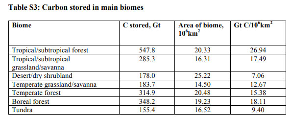
Sources: Carbon stored per biome: GRID Arendal, Area of biome

Observations indicate that the Amazon C sink decreased ~30% from 0.54 (0.45-0.63) Gt C/yr in the 1990s to 0.38 (0.28-0.49) Gt C/yr in the 2000s, partly due to increasing tree mortality linked to climate variability. Furthermore, individual drought events have reduced carbon uptake by 1.6 Gt C (2005) and 1.1 Gt C (2010) with the 2010 drought event making the Amazon essentially carbon neutral at 0.07 Gt C/yr. Extrapolation of the 0.16 Gt C/yr weakening of sink from the 1990s to 2000s for the remaining 83 years of this century gives a conservative minimum estimate of 13 Gt C equivalent emission from the Amazon, which we round to ~15 Gt C. Alternatively, assuming there continue to be on average two droughts per decade of comparable magnitude to the 2005 and 2010 events for the remaining eight decades of the century, the equivalent emission would be ~22 Gt C. This is in the range of the dieback estimates calculated above. Hence we consider ~25 Gt C to be a reasonable best estimate. Alternatively, if the observed rate of decline in Amazon C sink (0.016 Gt C/yr/yr)were to continue for the remainder of this century, then by the 2090s the Amazon would be a C source of 1.06 Gt C/yr and the equivalent carbon emission over the century would be ~80Gt C, or for the 83 years from 2017 onwards the equivalent emission would be ~55 Gt C. We take the latter as an upper estimate.

Boreal forest dieback

We estimate potential carbon loss from the dieback of the boreal forest from (i) extrapolation of observed changes (ii) model projections of dieback.1. Extrapolation from observed changes: Data from the Kurz and Apps (57) analysis of changes in the carbon budget for Canadian forests from 1920 to 1989 show an increase in carbon storage in biomass from 1920 to 1970 (11.0-16.4 Gt C), followed by a decrease from1970 to 1989 (16.4-14.5 Gt C), driven largely by an increase in disturbance regimes (insect induced stand mortality and fires) associated with a warming climate. DOM (Dead Organic Matter) showed an increase from 61.2 to 71.4 Gt C through the 70-year period. The increase in biomass and DOM over the 1920-1970 period is likely due, in part, to recovery from an earlier period of higher disturbance frequency.

If we assume that the rate of loss of biomass from 1970 to 1989 (1.9 Gt C through 20 years, or 0.095 Gt C per year) is maintained out to the end of the 21st century as the climate continues to warm, we estimate a loss of (0.095 Gt C/yr)(110 yrs) = 10.4 Gt C. Loss of about 10 Gt C over a century for the Canadian boreal forest is a reasonable (probably conservative)estimate when compared to an uptake in biomass of 5.4 Gt C through 50 years (from 1920 to1970) as the forest recovered from an earlier high disturbance regime. Assuming that the Canadian boreal forest comprises about one-third of the global boreal forest, gives a crude estimate of ~30 Gt C, for the amount of carbon that could be lost by 2100 from boreal forest dieback. These estimates are for biomass only and do not include increased C release from DOM as disturbance regimes change. Nevertheless, we take this as our central estimate.

A different analysis finds a 73% reduction in the strength of the C sink in boreal regions from 0.152 Gt C/yr in previous decades to 0.041 Gt C/yr over 1997-2006. Conservatively, if this 0.111 Gt C/yr reduction in sink strength persists over the subsequent 94 years to 2100 this corresponds to a C loss of 10.4 Gt C, in agreement with our Canada-only estimate above. Hence we take ~10 Gt C as our lower estimate. Alternatively, if the sink continues to decline at the observed rate 0.011 Gt C/yr/yr over 94 years this is equivalent to an emission of 49 Gt C, or for the 83 years from 2017 onwards the equivalent emission would be 38 Gt C. Hence we take ~40 Gt C as our upper estimate of the potential carbon loss through boreal forest dieback.

Model simulations of boreal forest conversion to savanna/grassland. The replacement of boreal forest at its southern boundary with steppe grasslands of lower carbon storage is consistent with grasslands being the neighbouring biome, as is an expansion of boreal forest into present-day tundra, which would increase carbon storage. Almost all models in the IPCC AR5 fail to capture the carbon dynamics of these biome transitions probably because they fail to appropriately capture disturbance factors. However, a novel estimate, based on ‘climate vectors’, of the equilibrium change in carbon storage expected under ~2°C warming (2040-2060 under RCP4.5) suggests a C loss over the 40-60°N region of 27 to 0.17 (mean 12.3) Gt C, but with an increase in C storage of 3.7-16 (mean 7.2) Gt C for the boreal forest transition.

Some earlier models also simulated boreal forest dieback, but both of these appear to simulate the ecosystem shifts at both the southern and northern edges of present-day boreal forests after they have reached equilibrium. Lucht et al. simulated a replacement of the boreal forest at its southern border in a large stretch across Siberia and to the southwest of Hudson Bay in Canada under a relatively high warming scenario, but they do not quantify the area of boreal forest dieback or the carbon lost. Joos et al. used a coupled climate-carbon cycle model to simulate changes in biome distribution and carbon dynamics using two emissions scenarios (moderate and high). For the moderate scenario, which gives a 2.8°C temperature rise by 2100, a large area of boreal forest in southern-central Siberia and a smaller area southwest of Hudson Bay in Canada are converted to savanna/woodland or grassland. This results in large losses of carbon in both areas (Plate 2 in their paper).Although Joos et al. do not report the carbon storage changes by biome, a rough approximation can be made based on an estimated 50% loss of boreal forest to savanna/grassland. Then based on Table S2, the carbon lost to the atmosphere by conversion of half of the global boreal forest to temperate savanna/grassland is

(19.23 106 km2 )(0.5) x (18.11-12.67 Gt C/106 km2) = 52.3 Gt C.

Assuming linear scaling with the level of temperature forcing would give an estimate of 52.3 Gt C (2.0/2.8) = 37.4 Gt C. This compares well with the upper estimate of 38 Gt C above based on Hayes et al..

The Koven, Lucht et al. and Joos et al. studies all simulate an uptake of carbon in the far north as boreal forests migrate into present-day tundra regions. However, none of the modelling studies appear to capture the century-scale lag between the rapid loss of carbon from disturbance-driven dieback and the much slower migration and growth of boreal forests into the higher latitudes. It is the pulse of carbon to the atmosphere resulting from this long lag time that we are estimating as the feedback resulting from boreal forest dieback(Table S1), an estimate we base on the observed carbon cycle dynamics of disturbance-driven dieback in the Canadian boreal forests. We emphasize that we are considering here the carbon dynamics of a highly transient phase of the Earth System (the potential ‘Hothouse Earth’ pathway) and one that is not close to equilibrium.

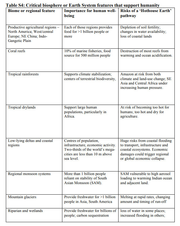
Critical biomes that support humanity (Section “What Is at Stake?” in the main text)

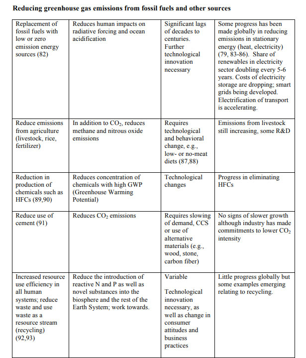
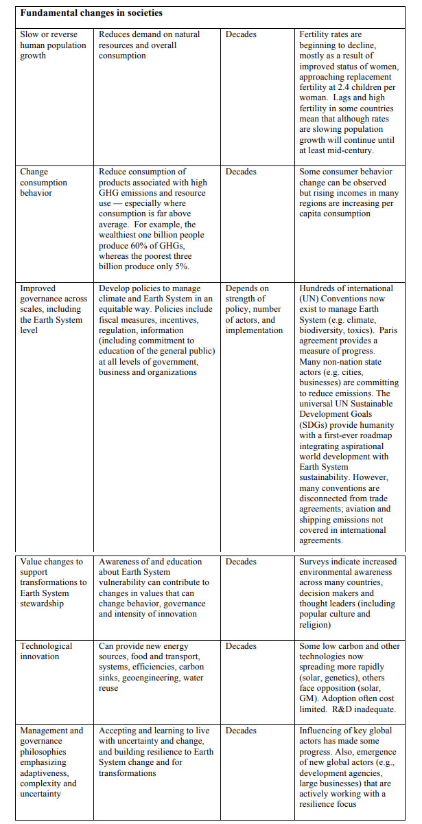
Human feedbacks in the Earth System (Section “Human Feedbacks in the Earth System” in the main text)

1 This carbon-sink feedback is fundamentally different from the others in that, in principle, it returns geological (fossil) carbon from the atmosphere to a geological formation, while the other sinks transfer carbon from one pool (atmosphere) to another (land or ocean) in the active carbon cycle. This carbon is vulnerable to return to the atmosphere whereas carbon stored safely in geological formations is not.